This notebook introduces basic polarimetric analysis using NISAR quad-polarization GSLC (Geocoded Single-Look Complex) products and polSARtools. Full-polarimetric GSLC data contain complex measurements from the HH, HV, VH, and VV polarization channels, enabling analysis of different scattering mechanisms. Using polSARtools, this notebook utilizes both scene-wide and subsetted examples to demonstrate how to:
extract the C3 covariance matrix
apply a Refined-Lee speckle filter
create a Pauli decomposition RGB composite
create a HH/HV/VV RGB composite
This example uses NISAR GSLC products, which provide geocoded complex SAR imagery suitable for polarimetric analysis and other advanced SAR applications. For more information on NISAR GSLC data, refer to the NISAR Data User Guide.
1. Prerequisites
| Prerequisite | Importance | Notes |
|---|---|---|
The isce3 software environment for this cookbook | Necessary | |
| How to search and access NISAR data in your AOI | Helpful | |
| Familiarity with polSARtools | Helpful | |
| General knowledge of polarimetry | Helpful |
Rough Notebook Time Estimate: 45 mins
2. Search and Download Dara
Use asf_search to find NISAR data.
2a. Search for Data and Identify an Area of Interest (AOI)
Use the interactive map below to generate well-known-text (WKT) of your AOI. Copy the wkt and update the area_of_interest variable in the next code cell.
import os
import asf_search as asf
from datetime import datetime
from getpass import getpass

import warnings
warnings.filterwarnings(
    "ignore",
    message="Parsing dates involving a day of month without a year specified",
)

# Option 1: Use Earthdata Login credentials stored in a .netrc file
session = asf.ASFSession()

# Option 2: Uncomment if needed: Enter your NASA Earthdata Login credentials
#session.auth_with_creds(input('EDL Username'), getpass('EDL Password'))

start_date = datetime(2026, 7, 3)
end_date = datetime(2026, 7, 5)

area_of_interest = "POLYGON((-147.762 64.8592,-147.6954 64.8592,-147.6954 64.8789,-147.762 64.8789,-147.762 64.8592))" # POINT or POLYGON as WKT (well-known-text)

pattern = r'^(?!.*QA_STATS).*'

opts=asf.ASFSearchOptions(**{
    "maxResults": 250,
    "intersectsWith": area_of_interest,
    "flightDirection": "DESCENDING",
    "start": start_date,
    "end": end_date,
    "processingLevel": ["GSLC"],
    "dataset": ["NISAR"],
    "productionConfiguration": ["PR"],
    "dataMaturity" : "PROVISIONAL",
    'session': session,
})

response = asf.search(opts=opts)
hdf5_urls = response.find_urls(extension='.h5', pattern=pattern, directAccess=False)
print(f"Found {len(hdf5_urls)} GSLC products:")
hdf5_urls
Found 1 GSLC products:
['https://nisar.asf.earthdatacloud.nasa.gov/NISAR/NISAR_L2_GSLC_PROVISIONAL_V1/NISAR_L2_PR_GSLC_024_116_D_055_2005_QPDH_A_20260704T055929_20260704T060006_P05023_N_F_J_001/NISAR_L2_PR_GSLC_024_116_D_055_2005_QPDH_A_20260704T055929_20260704T060006_P05023_N_F_J_001.h5']2b. Retain only the URL for the most recent version of each product in the search results
Data is occasionally re-released with an updated version. Versions are recorded as a Composite Release Identifier (CRID) in a product’s filename. We can use the CRID to retain only the most recent version of each product in the list of URLs.
import re

if len(hdf5_urls) == 1:
    print("Single GSLC product found. Skipping CRID filter.")

else:
    pattern = re.compile(
        r"(NISAR_L2_PR_GSLC.*?)_P([0-9]{5})_N_F_J_[0-9]{3}\.h5$")

    latest_version_dict = {}

    for url in hdf5_urls:
        fname = url.split("/")[-1]

        match = pattern.search(fname)

        if not match:
            print(f"No match: {fname}")
            continue

        product, crid = match.groups()

        if (
            product not in latest_version_dict
            or crid > latest_version_dict[product][0]
        ):
            latest_version_dict[product] = (crid, url)

    hdf5_urls = [item[1] for item in latest_version_dict.values()]

print(f"Retained {len(hdf5_urls)} GSLC products:")
hdf5_urls
Single GSLC product found. Skipping CRID filter.
Retained 1 GSLC products:
['https://nisar.asf.earthdatacloud.nasa.gov/NISAR/NISAR_L2_GSLC_PROVISIONAL_V1/NISAR_L2_PR_GSLC_024_116_D_055_2005_QPDH_A_20260704T055929_20260704T060006_P05023_N_F_J_001/NISAR_L2_PR_GSLC_024_116_D_055_2005_QPDH_A_20260704T055929_20260704T060006_P05023_N_F_J_001.h5']2c. Download the Data
%%time

from pathlib import Path

# Create a folder and download the files
data_dir = Path.home() / "polSAR_GSLC_data"
data_dir.mkdir(exist_ok=True)
print(f'data_dir: {data_dir}')

#download files
asf.download_urls(hdf5_urls, data_dir, session=session, processes=4)
data_dir: /home/jovyan/polSAR_GSLC_data
CPU times: user 161 μs, sys: 0 ns, total: 161 μs
Wall time: 156 μs
gslc_files = sorted(data_dir.glob("*.h5"))
gslc_files[PosixPath('/home/jovyan/polSAR_GSLC_data/NISAR_L2_PR_GSLC_024_116_D_055_2005_QPDH_A_20260704T055929_20260704T060006_P05023_N_F_J_001.h5')]3. Use polSARtools to Process Polarimetric Data
This notebook uses the polSARtools package to process and visualize full-polarization NISAR GSLC data. In the following sections, you’ll import the data, apply a speckle filter, and generate two commonly used RGB composites for interpretation.
# Select the first downloaded GSLC file
in_file = str(gslc_files[0])

print(in_file)
print(type(in_file))
/home/jovyan/polSAR_GSLC_data/NISAR_L2_PR_GSLC_024_116_D_055_2005_QPDH_A_20260704T055929_20260704T060006_P05023_N_F_J_001.h5
<class 'str'>
4. Extract C3 Covariance Matrix
NISAR GSLC products can be represented in several polarimetric matrix formats. In this notebook, we’ll extract the C3 covariance matrix, which contains the information needed to create both the Pauli RGB decomposition and the HH/HV/VV RGB composite.
Creating the C3 matrix directly from a GSLC with PolSARtools provides more control over processing choices such as multilooking and filtering. However, PolSARtools does not apply NISAR’s radiometric terrain correction when creating the matrix. If RTC is an important part of your analysis, consider using a GCOV product or manually creating a C3 matrix.
More about the C3 covariance matrix
The C3 covariance matrix is derived from the full-polarimetric scattering matrix and organizes the information from the HH, HV, and VV polarization channels into a 3 × 3 covariance matrix. In addition to preserving the scattering information from each channel, it describes how the polarization channels are related to one another, providing a more robust description of the scattering behavior that is less sensitive to random noise. This matrix serves as the foundation for several polarimetric processing techniques, including speckle filtering, visualization, decomposition, and classification.
The C3 covariance matrix has the following structure:
The diagonal elements (, , and ) describe the strength of the polarization components, while the off-diagonal elements describe the relationships between them. The indicates the complex conjugate of the corresponding element.
The C3 matrix can also be viewed in terms of the polarization combinations used to form it. Below, each C3 element shows either the strength of an individual polarization component or the relationship between two polarization components. The lower off-diagonal elements are complex conjugates of the corresponding upper elements.
import polsartools as pst

pst.import_nisar_gslc(
    in_file,
    mat="C3",
    azlks=20,
    rglks=10,
    fmt="tif",
    cog=False,
    ovr=[2, 4, 8, 16],
    comp=False,
    recip=False
)
5. Reduce Speckle with a Refined Lee Filter
Before creating RGB composites, apply the Refined Lee filter to reduce speckle while preserving important scattering features such as edges and boundaries. The implementation used by polsSARtools applies the same filter to all covariance terms, which is important for preserving the relationships between them while maintaining the ability to make relative comparisons between terms.
More about the Refined Lee Filter
The Refined Lee filter reduces speckle by analyzing the statistical properties of pixels in a local neighborhood. Rather than applying a fixed level of smoothing, it adjusts amounts of smoothing based on local image characteristics. The Refined Lee filter applies more smoothing in homogeneous areas while preserving edges, boundaries, and other important scattering features.
C3Folder = os.path.join(in_file.split(".h5")[0], "C3")

window_size = 3

pst.filter_refined_lee(
    C3Folder,
    win=window_size,
    fmt="tif",
    sub_dir=True,
    cog=False,
    ovr=[2, 4, 8, 16],
    comp=False
)
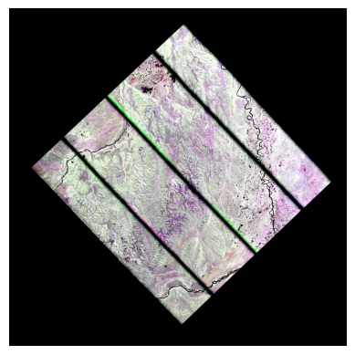
6. Create a Pauli RGB Composite
The Pauli decomposition combines the polarimetric channels to emphasize different scattering mechanisms:
Red: HH − VV (double-bounce scattering)
Green: HV (volume scattering)
Blue: HH + VV (surface scattering)
This composite is commonly used to distinguish scattering behavior across different land cover types.
filtered_C3 = os.path.join(
    in_file.split(".h5")[0],
    f"rlee_{window_size}x{window_size}",
    "C3"
)

pst.pauli_rgb(filtered_C3, save_tif=True)
Pauli RGB image saved as /home/jovyan/polSAR_GSLC_data/NISAR_L2_PR_GSLC_024_116_D_055_2005_QPDH_A_20260704T055929_20260704T060006_P05023_N_F_J_001/rlee_3x3/C3/PauliRGB.tif
Pauli RGB image saved as /home/jovyan/polSAR_GSLC_data/NISAR_L2_PR_GSLC_024_116_D_055_2005_QPDH_A_20260704T055929_20260704T060006_P05023_N_F_J_001/rlee_3x3/C3/PauliRGB.png
Execution time for pauli_rgb: 5.00 seconds
7. Create an HH/HV/VV RGB Composite
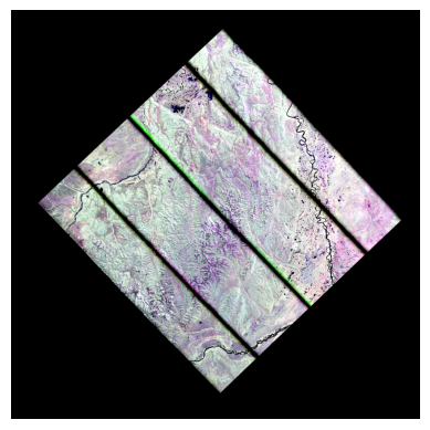
This composite assigns each polarization channel directly to a color:
Red: HH
Green: HV
Blue: VV
Unlike the Pauli decomposition, this visualization displays the relative backscatter intensity of each polarization channel without combining them into scattering mechanisms. It is useful for examining differences in vegetation structure, surface roughness, and moisture while preserving the original polarization information.
Comparing Composites
This notebook produces both a Pauli RGB Composite and a HH/HV/VV RGB Composite
Both images use polarimetric SAR information to create an RGB visualization, however, they display information differently.
The HH/HV/VV composite assigns individual polarization channels directly to the red, green, and blue channels. The resulting colors show differences in the relative strength of the HH, HV, and VV radar returns. This provides a relatively direct view of the measured polarimetric backscatter.
The Pauli composite does not assign the individual HH, HV, and VV channels directly to colors. Instead, it combines the polarization measurements into components that emphasize different scattering behaviors. This makes differences in scattering behavior easier to distinguish visually.
In summary, the HH/HV/VV composite shows the polarization measurements more directly, while the Pauli composite reorganizes those measurements to emphasize differences in how the radar signal interacts with the surface.
# Assign the HH, HV, and VV channels to the RGB channels
hh_path = next(Path(filtered_C3).glob("C11*.tif"))
hv_path = next(Path(filtered_C3).glob("C22*.tif"))
vv_path = next(Path(filtered_C3).glob("C33*.tif"))

# Create an RGB composite
pst.rgb(
    str(hh_path),  # Red: HH
    str(hv_path),  # Green: HV
    str(vv_path),  # Blue: VV
    norm_each=True,
    lp=5,
    gp=95,
    save_tif=True
)
RGB image saved as /home/jovyan/polSAR_GSLC_data/NISAR_L2_PR_GSLC_024_116_D_055_2005_QPDH_A_20260704T055929_20260704T060006_P05023_N_F_J_001/rlee_3x3/C3/RGB.png
RGB GeoTIFF saved as /home/jovyan/polSAR_GSLC_data/NISAR_L2_PR_GSLC_024_116_D_055_2005_QPDH_A_20260704T055929_20260704T060006_P05023_N_F_J_001/rlee_3x3/C3/RGB.tif
Execution time for rgb: 5.00 seconds
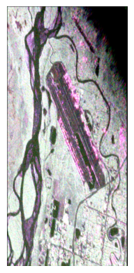
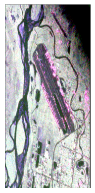
8. Create and Process a High Resolution Subset
The full-scene workflow provides an efficient way to process large GSLC products. When a smaller area of interest is sufficient, creating a spatial subset allows the data to be processed at a higher spatial resolution without extending processing times and storage requirements. The following sections repeat the same polarimetric processing workflow using a subsetted GSLC.
8.1. Create a Subset
polsartools expects a standard NISAR GSLC HDF5 product as input. Here, we create a subset that preserves the original HDF5 structure and metadata.
%%time
import sys
project_root = Path.cwd().parent
sys.path.insert(0, str(project_root))

from util.subset_h5 import subset_h5

area_of_interest = "POLYGON((-147.9245 64.7827,-147.779 64.7827,-147.779 64.8382,-147.9245 64.8382,-147.9245 64.7827))" # desired AOI for subset

subset_file = subset_h5(
    in_file,
    area_of_interest,
)

print(subset_file)
/home/jovyan/polSAR_GSLC_data/subset/NISAR_L2_PR_GSLC_024_116_D_055_2005_QPDH_A_20260704T055929_20260704T060006_P05023_N_F_J_001_subset.h5
CPU times: user 410 ms, sys: 360 ms, total: 770 ms
Wall time: 770 ms
8.2 Extract the C3 Covariance Matrix
subset_in_file = str(subset_file)

pst.import_nisar_gslc(
    subset_in_file,
    mat="C3",
    azlks=2,
    rglks=2,
    fmt="tif",
    cog=False,
    ovr=[2, 4, 8, 16],
    comp=False,
    recip=False
)
Detected L-band polarization channels: ['HH' 'HV' 'VH' 'VV']
Extracting C3 matrix elements...
Processing chunks: 100%|██████████| 8/8 [00:00<00:00, 48.27it/s]
Saved file /home/jovyan/polSAR_GSLC_data/subset/NISAR_L2_PR_GSLC_024_116_D_055_2005_QPDH_A_20260704T055929_20260704T060006_P05023_N_F_J_001_subset/C3/C11.tif
Saved file /home/jovyan/polSAR_GSLC_data/subset/NISAR_L2_PR_GSLC_024_116_D_055_2005_QPDH_A_20260704T055929_20260704T060006_P05023_N_F_J_001_subset/C3/C12_real.tif
Saved file /home/jovyan/polSAR_GSLC_data/subset/NISAR_L2_PR_GSLC_024_116_D_055_2005_QPDH_A_20260704T055929_20260704T060006_P05023_N_F_J_001_subset/C3/C12_imag.tif
Saved file /home/jovyan/polSAR_GSLC_data/subset/NISAR_L2_PR_GSLC_024_116_D_055_2005_QPDH_A_20260704T055929_20260704T060006_P05023_N_F_J_001_subset/C3/C13_real.tif
Saved file /home/jovyan/polSAR_GSLC_data/subset/NISAR_L2_PR_GSLC_024_116_D_055_2005_QPDH_A_20260704T055929_20260704T060006_P05023_N_F_J_001_subset/C3/C13_imag.tif
Saved file /home/jovyan/polSAR_GSLC_data/subset/NISAR_L2_PR_GSLC_024_116_D_055_2005_QPDH_A_20260704T055929_20260704T060006_P05023_N_F_J_001_subset/C3/C22.tif
Saved file /home/jovyan/polSAR_GSLC_data/subset/NISAR_L2_PR_GSLC_024_116_D_055_2005_QPDH_A_20260704T055929_20260704T060006_P05023_N_F_J_001_subset/C3/C23_real.tif
Saved file /home/jovyan/polSAR_GSLC_data/subset/NISAR_L2_PR_GSLC_024_116_D_055_2005_QPDH_A_20260704T055929_20260704T060006_P05023_N_F_J_001_subset/C3/C23_imag.tif
Saved file /home/jovyan/polSAR_GSLC_data/subset/NISAR_L2_PR_GSLC_024_116_D_055_2005_QPDH_A_20260704T055929_20260704T060006_P05023_N_F_J_001_subset/C3/C33.tif
Execution time for import_nisar_gslc: 0.00 seconds
8.3 Reduce Speckle with the Refined Lee Filter
subset_C3Folder = os.path.join(
    subset_in_file.split(".h5")[0],
    "C3"
)
subset_window_size = 3

pst.filter_refined_lee(
    subset_C3Folder,
    win=subset_window_size,
    fmt="tif",
    sub_dir=True,
    cog=False,
    ovr=[2, 4, 8, 16],
    comp=False
)
Progress: 100%|██████████| 2/2 [00:01<00:00, 1.88block/s]Saved file /home/jovyan/polSAR_GSLC_data/subset/NISAR_L2_PR_GSLC_024_116_D_055_2005_QPDH_A_20260704T055929_20260704T060006_P05023_N_F_J_001_subset/rlee_3x3/C3/C11.tif
Saved file /home/jovyan/polSAR_GSLC_data/subset/NISAR_L2_PR_GSLC_024_116_D_055_2005_QPDH_A_20260704T055929_20260704T060006_P05023_N_F_J_001_subset/rlee_3x3/C3/C12_real.tif
Saved file /home/jovyan/polSAR_GSLC_data/subset/NISAR_L2_PR_GSLC_024_116_D_055_2005_QPDH_A_20260704T055929_20260704T060006_P05023_N_F_J_001_subset/rlee_3x3/C3/C12_imag.tif
Saved file /home/jovyan/polSAR_GSLC_data/subset/NISAR_L2_PR_GSLC_024_116_D_055_2005_QPDH_A_20260704T055929_20260704T060006_P05023_N_F_J_001_subset/rlee_3x3/C3/C13_real.tif
Saved file /home/jovyan/polSAR_GSLC_data/subset/NISAR_L2_PR_GSLC_024_116_D_055_2005_QPDH_A_20260704T055929_20260704T060006_P05023_N_F_J_001_subset/rlee_3x3/C3/C13_imag.tif
Saved file /home/jovyan/polSAR_GSLC_data/subset/NISAR_L2_PR_GSLC_024_116_D_055_2005_QPDH_A_20260704T055929_20260704T060006_P05023_N_F_J_001_subset/rlee_3x3/C3/C22.tif
Saved file /home/jovyan/polSAR_GSLC_data/subset/NISAR_L2_PR_GSLC_024_116_D_055_2005_QPDH_A_20260704T055929_20260704T060006_P05023_N_F_J_001_subset/rlee_3x3/C3/C23_real.tif
Saved file /home/jovyan/polSAR_GSLC_data/subset/NISAR_L2_PR_GSLC_024_116_D_055_2005_QPDH_A_20260704T055929_20260704T060006_P05023_N_F_J_001_subset/rlee_3x3/C3/C23_imag.tif
Saved file /home/jovyan/polSAR_GSLC_data/subset/NISAR_L2_PR_GSLC_024_116_D_055_2005_QPDH_A_20260704T055929_20260704T060006_P05023_N_F_J_001_subset/rlee_3x3/C3/C33.tif
Execution time for filter_refined_lee: 1.00 seconds
8.4 Create a Pauli RGB Composite
filtered_subset_C3 = os.path.join(
    subset_in_file.split(".h5")[0],
    f"rlee_{subset_window_size}x{subset_window_size}",
    "C3"
)

pst.pauli_rgb(filtered_subset_C3, save_tif=True)
Pauli RGB image saved as /home/jovyan/polSAR_GSLC_data/subset/NISAR_L2_PR_GSLC_024_116_D_055_2005_QPDH_A_20260704T055929_20260704T060006_P05023_N_F_J_001_subset/rlee_3x3/C3/PauliRGB.tif
Pauli RGB image saved as /home/jovyan/polSAR_GSLC_data/subset/NISAR_L2_PR_GSLC_024_116_D_055_2005_QPDH_A_20260704T055929_20260704T060006_P05023_N_F_J_001_subset/rlee_3x3/C3/PauliRGB.png
Execution time for pauli_rgb: 0.00 seconds
8.5 Create an HH/HV/VV RGB Composite
# Assign the HH, HV, and VV channels to the RGB channels
hh_path = next(Path(filtered_subset_C3).glob("C11*.tif"))
hv_path = next(Path(filtered_subset_C3).glob("C22*.tif"))
vv_path = next(Path(filtered_subset_C3).glob("C33*.tif"))

# Create an HH/HV/VV RGB composite
pst.rgb(
    str(hh_path),  # Red: HH
    str(hv_path),  # Green: HV
    str(vv_path),  # Blue: VV
    norm_each=True,
    lp=5,
    gp=95,
    save_tif=True
)
RGB image saved as /home/jovyan/polSAR_GSLC_data/subset/NISAR_L2_PR_GSLC_024_116_D_055_2005_QPDH_A_20260704T055929_20260704T060006_P05023_N_F_J_001_subset/rlee_3x3/C3/RGB.png
RGB GeoTIFF saved as /home/jovyan/polSAR_GSLC_data/subset/NISAR_L2_PR_GSLC_024_116_D_055_2005_QPDH_A_20260704T055929_20260704T060006_P05023_N_F_J_001_subset/rlee_3x3/C3/RGB.tif
Execution time for rgb: 0.00 seconds
9. Visualize the Scene-Wide and Subsetted Composites on an Interactive Map
polSARtools allows RGB composites to easily be saved as GeoTIFFs. Here, the both the scene-wide images and the higher-resolution subset are overlaid on a basemap to provide geographic context for the observed scattering patterns.
# Scene-wide GeoTIFFs
scene_pauli_tif = Path(filtered_C3) / "PauliRGB.tif"
scene_rgb_tif = Path(filtered_C3) / "RGB.tif"

# High res subsetted GeoTIFFs
subset_pauli_tif = Path(filtered_subset_C3) / "PauliRGB.tif"
subset_rgb_tif = Path(filtered_subset_C3) / "RGB.tif"
import numpy as np
import rasterio
from rasterio.warp import calculate_default_transform, reproject, Resampling
def prepare_rgb_overlay(tif_path):
with rasterio.open(tif_path) as src:
transform, width, height = calculate_default_transform(
src.crs,
"EPSG:4326",
src.width,
src.height,
*src.bounds,
)
rgb = np.zeros((3, height, width), dtype=np.uint8)
for band in range(3):
reproject(
source=rasterio.band(src, band + 1),
destination=rgb[band],
src_transform=src.transform,
src_crs=src.crs,
dst_transform=transform,
dst_crs="EPSG:4326",
resampling=Resampling.nearest,
)
rgb = np.moveaxis(rgb, 0, -1)
# Make pixels with no RGB values transparent
alpha = np.where(np.any(rgb > 0, axis=2), 255, 0).astype(np.uint8)
rgba = np.dstack((rgb, alpha))
west = transform.c
north = transform.f
east = west + transform.a * width
south = north + transform.e * height
bounds = [[south, west], [north, east]]
return rgba, boundsscene_pauli_img, scene_pauli_bounds = prepare_rgb_overlay(scene_pauli_tif)
scene_rgb_img, scene_rgb_bounds = prepare_rgb_overlay(scene_rgb_tif)
subset_pauli_img, subset_pauli_bounds = prepare_rgb_overlay(subset_pauli_tif)
subset_rgb_img, subset_rgb_bounds = prepare_rgb_overlay(subset_rgb_tif)import folium
m = folium.Map(
tiles="Esri.WorldImagery",
)
folium.raster_layers.ImageOverlay(
image=scene_pauli_img,
bounds=scene_pauli_bounds,
name="Scene-wide Pauli RGB",
opacity=0.8,
show=True,
).add_to(m)
folium.raster_layers.ImageOverlay(
image=scene_rgb_img,
bounds=scene_rgb_bounds,
name="Scene-wide HH/HV/VV RGB",
opacity=0.8,
show=False,
).add_to(m)
folium.raster_layers.ImageOverlay(
image=subset_pauli_img,
bounds=subset_pauli_bounds,
name="Subset Pauli RGB",
opacity=0.9,
show=False,
).add_to(m)
folium.raster_layers.ImageOverlay(
image=subset_rgb_img,
bounds=subset_rgb_bounds,
name="Subset HH/HV/VV RGB",
opacity=0.9,
show=False,
).add_to(m)
folium.LayerControl(collapsed=False).add_to(m)
m.fit_bounds(scene_pauli_bounds)
m10. Summary
You have now learned how to process full-polarimetric NISAR GSLC data using polsartools. This workflow demonstrated how to extract the C3 covariance matrix, reduce speckle with the Refined Lee filter, generate Pauli RGB and HH/HV/VV RGB composites, and create a high resolution spatial subset for more detailed polarimetric analysis.
Note: This workflow processes NISAR GSLC data for polarimetric analysis, but it does not perform radiometric terrain correction or create a GCOV-equivalent product. Users who require radiometrically terrain-corrected backscatter should consider using a NISAR GCOV product.