This notebook demonstrates how to generate an interferogram from a pair of NISAR Geocoded Single-Look Complex (GSLC) products. The workflow includes searching for data, accessing GSLCs through downloading or cloud streaming, selecting a polarization, defining an (optional) area of interest, generating an interferogram, visualizing the resulting wrapped phase, and exporting files.
This example uses NISAR GSLC products, which provide geocoded complex SAR imagery suitable for interferometric analysis and other advanced SAR applications. The NISAR data in this notebook captures the eruption of Ethiopia’s Hayli Gubbi Volcano on November 23, 2025. For more information on the eruption, follow this link. For more information on NISAR GSLC data, refer to the NISAR Data User Guide.
More Information on Interferometry
Interferometry compares the phase of two SAR images acquired over the same area at different times. This notebook demonstrates one of the simplest approaches for creating an interferogram from a pair of NISAR GSLC products: multiplying one complex image by the complex conjugate of another.
The resulting interferogram contains wrapped phase values ranging from to . These phase differences may be caused by topography, surface displacement, atmospheric effects, or changes in scattering properties between acquisitions.
This example focuses on generating and visualizing a wrapped interferogram and is intended as an introduction to interferometric processing with NISAR GSLC products.
1. Prerequisites
| Prerequisite | Importance | Notes |
|---|---|---|
The isce3 software environment for this cookbook | Necessary | |
| How to search and access NISAR data in your AOI | Necessary | If you wish to process data in your AOI instead of the example data |
| Familiarity with xarray | Helpful | |
| General knowledge of interferometry | Helpful |
Rough Notebook Time Estimate: 15 mins
2. Search for data
Use asf_search to find GSLC data.
2a. Perform an asf_search.search() to identify your desired product URLs
import os
import asf_search as asf
from datetime import datetime
from getpass import getpass

import warnings
warnings.filterwarnings(
    "ignore",
    message="Parsing dates involving a day of month without a year specified",
)

session = asf.ASFSession()

start_date = datetime(2025, 11, 21)
end_date = datetime(2025, 12, 7)
area_of_interest = "POLYGON((40.1106 12.4104,41.8474 12.4104,41.8474 14.2538,40.1106 14.2538,40.1106 12.4104))" # POINT or POLYGON as WKT (well-known-text)
pattern = r'^(?!.*QA_STATS).*'

opts=asf.ASFSearchOptions(**{
    "maxResults": 250,
    "intersectsWith": area_of_interest,
    "flightDirection": "ASCENDING",
    "start": start_date,
    "end": end_date,
    "relativeOrbit": 172,
    "frame": 8,
    "processingLevel": [
        "GSLC"
    ],
    "dataset": [
        "NISAR"
    ],
    "productionConfiguration": [
        "PR"
    ],
    'session': session,
})

response = asf.search(opts=opts)
hdf5_urls = response.find_urls(extension='.h5', pattern=pattern, directAccess=False)
print(f"Found {len(hdf5_urls)} GSLC products:")
hdf5_urls
Found 4 GSLC products:
['https://nisar.asf.earthdatacloud.nasa.gov/NISAR/NISAR_L2_GSLC_BETA_V1/NISAR_L2_PR_GSLC_005_172_A_008_2005_DHDH_A_20251122T024618_20251122T024652_X05007_N_F_J_001/NISAR_L2_PR_GSLC_005_172_A_008_2005_DHDH_A_20251122T024618_20251122T024652_X05007_N_F_J_001.h5',
 'https://nisar.asf.earthdatacloud.nasa.gov/NISAR/NISAR_L2_GSLC_BETA_V1/NISAR_L2_PR_GSLC_005_172_A_008_2005_DHDH_A_20251122T024618_20251122T024652_X05009_N_F_J_001/NISAR_L2_PR_GSLC_005_172_A_008_2005_DHDH_A_20251122T024618_20251122T024652_X05009_N_F_J_001.h5',
 'https://nisar.asf.earthdatacloud.nasa.gov/NISAR/NISAR_L2_GSLC_BETA_V1/NISAR_L2_PR_GSLC_006_172_A_008_2005_DHDH_A_20251204T024618_20251204T024653_X05007_N_F_J_001/NISAR_L2_PR_GSLC_006_172_A_008_2005_DHDH_A_20251204T024618_20251204T024653_X05007_N_F_J_001.h5',
 'https://nisar.asf.earthdatacloud.nasa.gov/NISAR/NISAR_L2_GSLC_BETA_V1/NISAR_L2_PR_GSLC_006_172_A_008_2005_DHDH_A_20251204T024618_20251204T024653_X05009_N_F_J_001/NISAR_L2_PR_GSLC_006_172_A_008_2005_DHDH_A_20251204T024618_20251204T024653_X05009_N_F_J_001.h5']
2b. Retain only the URL for the most recent version of each product in the search results
Data is occasionally re-released with an updated version. Versions are recorded as a Composite Release Identifier (CRID) in a product’s filename. We can use the CRID to retain only the most recent version of each product in the list of URLs.
import re

pattern = re.compile(
    r"(NISAR_L2_PR_GSLC.*?)_X([0-9]{5})_N_F_J_[0-9]{3}\.h5$"
)

latest_version_dict = {}

for url in hdf5_urls:
    fname = url.split("/")[-1]

    m = pattern.search(fname)
    if not m:
        print(f"No match: {fname}")
        continue

    product, crid = m.groups()

    if product not in latest_version_dict or crid > latest_version_dict[product][0]:
        latest_version_dict[product] = (crid, url)

hdf5_urls = [i[1] for i in latest_version_dict.values()]

print(f"Retained {len(hdf5_urls)} GSLC products:")
hdf5_urls
Retained 2 GSLC products:
['https://nisar.asf.earthdatacloud.nasa.gov/NISAR/NISAR_L2_GSLC_BETA_V1/NISAR_L2_PR_GSLC_005_172_A_008_2005_DHDH_A_20251122T024618_20251122T024652_X05009_N_F_J_001/NISAR_L2_PR_GSLC_005_172_A_008_2005_DHDH_A_20251122T024618_20251122T024652_X05009_N_F_J_001.h5',
 'https://nisar.asf.earthdatacloud.nasa.gov/NISAR/NISAR_L2_GSLC_BETA_V1/NISAR_L2_PR_GSLC_006_172_A_008_2005_DHDH_A_20251204T024618_20251204T024653_X05009_N_F_J_001/NISAR_L2_PR_GSLC_006_172_A_008_2005_DHDH_A_20251204T024618_20251204T024653_X05009_N_F_J_001.h5']
3. Select Data Access Options
This notebook can be run locally or on OpenScienceLab. Users may either download the GSLC files or stream them directly from the cloud. If running locally, consider streaming data with HTTPS to avoid downloading large GSLC files.
3a. Option 1: Download the data
from pathlib import Path

# Create a folder and download the files
data_dir = Path.home() / "GSLC_data"
data_dir.mkdir(exist_ok=True)
print(f'data_dir: {data_dir}')

#download files
asf.download_urls(hdf5_urls, data_dir, session=session, processes=4)
data_dir: /home/jovyan/GSLC_data
gslc_files = sorted(data_dir.glob("*.h5"))
gslc_files
[PosixPath('/home/jovyan/GSLC_data/NISAR_L2_PR_GSLC_005_172_A_008_2005_DHDH_A_20251122T024618_20251122T024652_X05009_N_F_J_001.h5'),
PosixPath('/home/jovyan/GSLC_data/NISAR_L2_PR_GSLC_006_172_A_008_2005_DHDH_A_20251204T024618_20251204T024653_X05009_N_F_J_001.h5')]3b. Option 2: Stream Data with HTTPS
Provide your Earthdata Login (EDL) Bearer Token
HTTPS requires an EDL Bearer Token
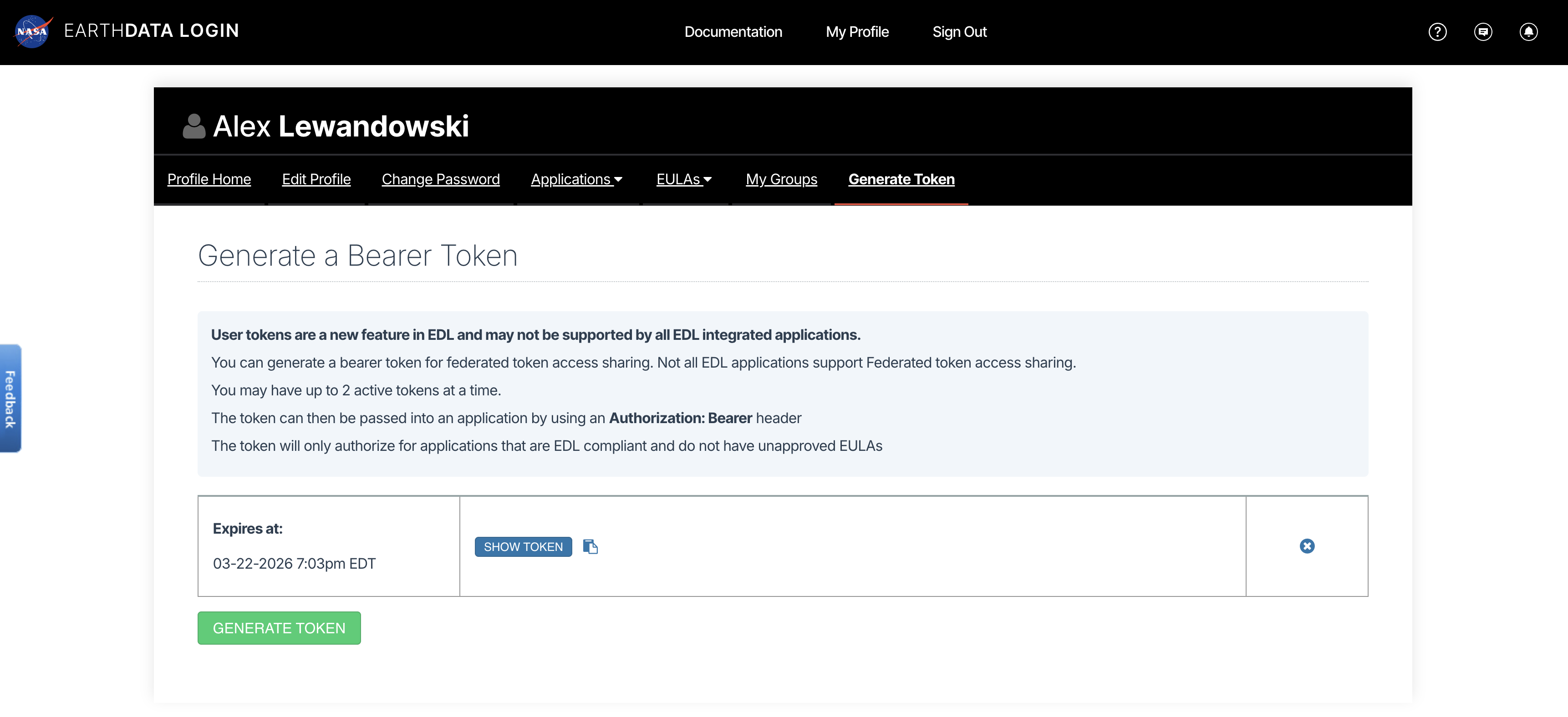
View or generate a Bearer Token in “Generate Token” tab of the Profile page in your Earthdata Login account: https://
from getpass import getpass

token = getpass("Enter your EDL Bearer Token")
%%time
import fsspec
import xarray as xr
fs = fsspec.filesystem(
"http",
headers={"Authorization": f"Bearer {token}"},
)
group_path = "/science/LSAR/GSLC/grids/frequencyA"
kwargs = {
"cache_type": "background",
"block_size": 8 * 1024 * 1024, # 8 MB
}
gslc_files = [
fs.open(url, "rb", **kwargs)
for url in hdf5_urls
]4. Open and inspect GSLCs
Open each GSLC as an xarray.DataTree to inspect the files and view available polarizations
import xarray as xr

gslc_dt = [
    xr.open_datatree(
        f,
        engine="h5netcdf",
        decode_timedelta=False,
        phony_dims="access",
        chunks="auto",
        group="/science/LSAR/GSLC/grids/frequencyA",
    )
    for f in gslc_files
]gslc_dt[0]gslc_dt[1]5. Select Input Data
Prepare the interferogram by:
Selecting a polarization
Choosing the reference (primary) GSLC
Choosing the secondary GSLC
Defining a spatial subset (optional)
5a. Select a polarization and view data
Available polarizations can be viewed in either xarray.DataTree in Section 4.
pol = "HH"5b. Assign Primary and Secondary Files
ref_file = gslc_dt[0][pol]
sec_file = gslc_dt[1][pol]
6. Define and Visualize a Subset
Optionally define a spatial subset to reduce processing time and focus the analysis on a specific area of interest. The subset can be specified using a WKT polygon and visualized before generating the interferogram. To draw and copy/paste a WKT, use the AOI “Draw a Box” tool on the ASF Data Search website.
#define epsg for subsetting and writing exports

epsg = int(gslc_dt[0].projection.attrs["epsg_code"])

epsg32637#define area of interest
wkt = "POLYGON((40.5327 13.4179,40.8702 13.4179,40.8702 13.7066,40.5327 13.7066,40.5327 13.4179))"import rioxarray
from shapely import wkt as shapely_wkt
from rasterio.warp import transform_bounds
epsg = int(gslc_dt[0].projection.attrs["epsg_code"])
crs = f"EPSG:{epsg}"
ref_file = ref_file.rio.write_crs(crs)
sec_file = sec_file.rio.write_crs(crs)
geom = shapely_wkt.loads(wkt)
bounds = transform_bounds(
"EPSG:4326",
crs,
*geom.bounds
)
ref_subset = ref_file.rio.clip_box(*bounds)
sec_subset = sec_file.rio.clip_box(*bounds)import matplotlib.pyplot as plt
from pyproj import Transformer
import contextily as cx
# Bounds from rioxarray
xmin, ymin, xmax, ymax = ref_file.rio.bounds()
axmin, aymin, axmax, aymax = ref_subset.rio.bounds()
transformer = Transformer.from_crs(
ref_file.rio.crs,
"EPSG:3857",
always_xy=True
)
# Transform bounds
xmin_wm, ymin_wm = transformer.transform(xmin, ymin)
xmax_wm, ymax_wm = transformer.transform(xmax, ymax)
axmin_wm, aymin_wm = transformer.transform(axmin, aymin)
axmax_wm, aymax_wm = transformer.transform(axmax, aymax)
fig, ax = plt.subplots(figsize=(10, 10))
ax.plot(
[xmin_wm, xmax_wm, xmax_wm, xmin_wm, xmin_wm],
[ymin_wm, ymin_wm, ymax_wm, ymax_wm, ymin_wm],
linewidth=2,
color="yellow",
label="Full raster"
)
ax.plot(
[axmin_wm, axmax_wm, axmax_wm, axmin_wm, axmin_wm],
[aymin_wm, aymin_wm, aymax_wm, aymax_wm, aymin_wm],
linewidth=3,
color="red",
label="Subset AOI"
)
cx.add_basemap(
ax,
source=cx.providers.Esri.WorldImagery,
)
ax.legend(loc="upper right")
ax.set_axis_off()
plt.show()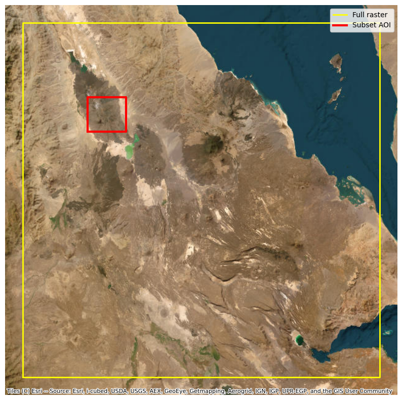
7. Create and Visualize a Subsetted Interferogram
In this section, the reference and secondary GSLCs are combined to generate an interferogram for the selected area of interest.
7a. Form the Subsetted Interferogram
Create the interferogram by multiplying the reference GSLC by the complex conjugate of the secondary GSLC. This preserves the phase difference between the two acquisitions.
import numpy as np

ifg_subset = ref_subset * np.conj(sec_subset)

ifg_subset7b. Extract the Interferometric Phase
The interferogram is a complex-valued dataset. To visualize phase differences, compute the phase angle of each pixel. Phase values are wrapped to the range to .
phase_subset = xr.apply_ufunc(
    np.angle,
    ifg_subset,
    dask="allowed",
)
7c. Visualize the Wrapped Subsetted Interferogram
Display the wrapped interferometric phase. Areas with similar colors have similar phase values, while rapid color transitions indicate strong phase gradients or deformation signals.
phase_subset.plot.imshow(
    cmap="jet",
    vmin=-np.pi,
    vmax=np.pi,
    size=10,
    cbar_kwargs={"label": "Phase (radians)"}
)

plt.title("Wrapped Subsetted Interferogram")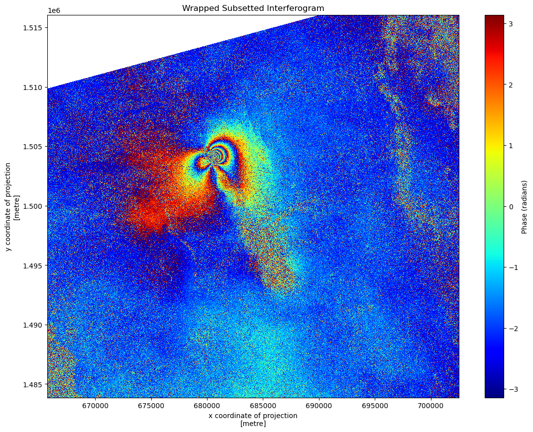
8. Create and Visualize a Scene-Wide Interferogram
In this section, the reference and secondary GSLCs are combined to generate an interferogram for entire NISAR scene. Note that processing times will be longer for this section due to the large size of NISAR GSLC files.
8a. Form the Scene-Wide Interferogram
Create the interferogram by multiplying the reference GSLC by the complex conjugate of the secondary GSLC. This preserves the phase difference between the two acquisitions.
ifg_scene = ref_file * np.conj(sec_file)

ifg_scene8b. Compute the Full-Resolution Interferometric Phase
The full-resolution interferogram is large and can be slow to display. For visualization, we multilook the interferogram by averaging blocks of complex pixels. This reduces noise and decreases the dataset size before plotting. Because interferometric phase is circular, the complex interferogram is averaged before computing the phase angle.
phase_scene = xr.apply_ufunc(
    np.angle,
    ifg_scene,
    dask="allowed",
)
8c. Multilook and Visualize the Scene-Wide Interferogram
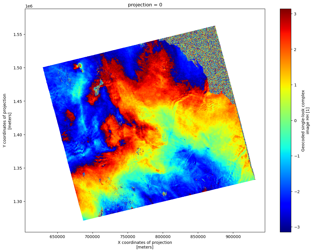
Displaying the full-resolution scene can be slow, especially when streaming data over HTTPS. For visualization, the complex interferogram is multilooked by averaging groups of neighboring pixels before computing the phase. This reduces noise and the amount of data that must be displayed while preserving the circular nature of the phase.
If plotting is slow, increase the coarsening factors (yCoordinates and xCoordinates) below. Larger values will display more quickly but will reduce spatial detail.
%%time
# multilook
phase_multilook = ifg_scene.coarsen(
    yCoordinates=10,
    xCoordinates=10,
    boundary="trim"
).mean()

# Find phase angles
phase_multilook_radians = xr.apply_ufunc(
    np.angle,
    phase_multilook,
    dask="allowed",
)

# plot
phase_multilook_radians.plot.imshow(
    cmap="jet",
    vmin=-np.pi,
    vmax=np.pi,
    size=10
)
CPU times: user 1min 31s, sys: 28.2 s, total: 1min 59s
Wall time: 2min 25s
9. Export Files
The interferograms generated in this notebook can be exported for use in GIS software, additional processing workflows, or archival purposes. This section demonstrates how to save both the subsetted and scene-wide interferograms as GeoTIFF and/or HDF5 files.
Note: To open the following h5 files in QGIS, rename the “.h5” extension to “nc.” For more information, see the Using NISAR Data section of the NISAR Data User Guide.
Write crs before exporting
phase_subset_export = phase_subset.rio.write_crs(f"EPSG:{epsg}")phase_scene_export = phase_scene.rio.write_crs(f"EPSG:{epsg}")9a. Export Subsetted Interferogram as GeoTIFF
phase_subset_export.rio.to_raster(
    "phase_subset.tif",
    compress="deflate"
)
9b. Export Subsetted Interferogram as h5
phase_subset_export.to_netcdf(
    "phase_subset.h5",
    engine="h5netcdf"
)
9c. Export Scene-Wide Interferogram as GeoTIFF
%%time
phase_scene_export.rio.to_raster(
    "phase_scene.tif",
    driver="GTiff",
    tiled=True,
    windowed=True,
    BIGTIFF="YES",
)
CPU times: user 6h 13min 39s, sys: 27min 32s, total: 6h 41min 11s
Wall time: 6h 41min 46s
9d. Export Scene-Wide Interferogram as h5
%%time
# ~8MB chunks
phase_scene_h5 = phase_scene.chunk({
    "yCoordinates": 1440,
    "xCoordinates": 1440
})

phase_scene_h5.to_netcdf(
    "phase_scene.h5",
    engine="h5netcdf"
)
CPU times: user 1min 46s, sys: 55.1 s, total: 2min 41s
Wall time: 5min 44s
10. Summary
You have now learned how to generate an interferogram using a pair of NISAR GSLC products. This workflow demonstrated how to access GSLC data, select a polarization and area of interest, create and visualize a wrapped interferogram, and export the results for use in downstream analyses.
11. Resources and references
Author: Julia White, Alex Lewandowski